
Introduction to Graph Clustering
Last updated: Friday June 27th, 2025
Report this blog
Previously I wrote a blog on how to divide the countries of the world into 10 even groups. While I did the grouping manually and intuitively, I wonder if there is a more scientific way to do the same. After some research, there are indeed many methodologies in doing similar task. In this blog, I will go through some of these.
Before we begin, let me explain some basic terminology in the science of map and grouping:
- Vector: a list of numbers.
- Matrix: a table of numbers.
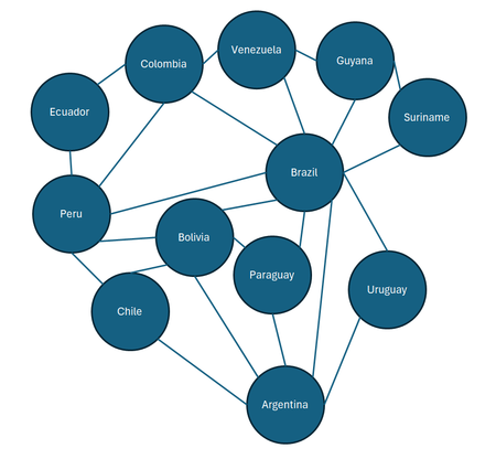
- Graph: a group of related and connected objects. In our case, it is the world map.
- Vertex or node: the object in a graph, e.g. the numbered circles in the diagram below. In our case, these are the countries.
- Edge: the line connecting the vertices. In our case, these can be the country borders.
- Clustering: the process of grouping nodes, which is what I am trying to do here.

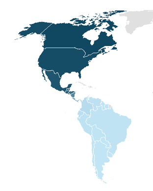
To explain the different methods, in this blog I will attempt to divide the South American countries into two groups. South America is used because it is relatively simple with only 12 countries (excluding France), and there are no island countries (because for island countries we need to decide how to set the edges, more on that later).
Hierarchical Clustering
Hierarchical clustering is to build clusters like a family tree. It can either starts bottom-up by merging smaller clusters into larger ones, or top-down by breaking down large clusters into smaller ones. Here I will use the first method on the South American countries.
First treat the 12 countries as 12 clusters, and calculate the distance between each of them (I am using the capitals here).
| AR | BO | BR | CL | CO | EC | GY | PY | PE | SR | UY | VE | |
|---|---|---|---|---|---|---|---|---|---|---|---|---|
| Argentina | 0 | |||||||||||
| Bolivia | 2235 | 0 | ||||||||||
| Brazil | 2340 | 2160 | 0 | |||||||||
| Chile | 1135 | 1902 | 3009 | 0 | ||||||||
| Colombia | 4660 | 2436 | 3664 | 4248 | 0 | |||||||
| Ecuador | 4357 | 2137 | 3776 | 3785 | 730 | 0 | ||||||
| Guyana | 4605 | 2815 | 2752 | 4667 | 1779 | 2391 | 0 | |||||
| Paraguay | 1037 | 1465 | 1462 | 1551 | 3770 | 3578 | 3570 | 0 | ||||
| Peru | 3136 | 1077 | 3165 | 2468 | 1880 | 1324 | 2958 | 2513 | 0 | |||
| Suriname | 4513 | 2868 | 2535 | 4667 | 2099 | 2680 | 346 | 3476 | 3132 | 0 | ||
| Uruguay | 206 | 2361 | 2272 | 1340 | 4770 | 4494 | 4635 | 1069 | 3294 | 4527 | 0 | |
| Venezuela | 5093 | 3004 | 3589 | 4903 | 1028 | 1755 | 1043 | 4104 | 2745 | 1387 | 5164 | 0 |
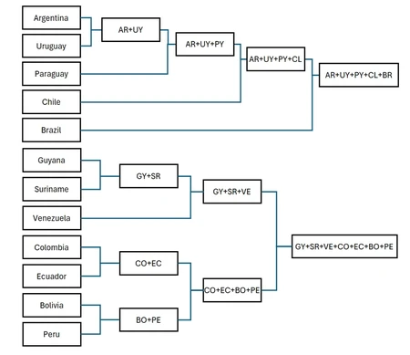
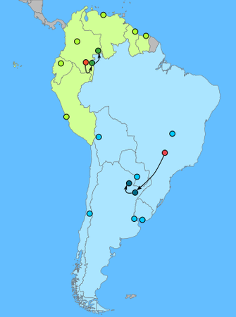
It turns out that Argentina (Buenos Aires) and Uruguay (Montevideo) are the closest together, so let's merge them to form a new cluster. Now, recentre Argentina + Uruguay and recalculate the distance between it and the remaining nodes:
| BO | BR | CL | CO | EC | GY | PY | PE | SR | VE | AR+UY | |
|---|---|---|---|---|---|---|---|---|---|---|---|
| Argentina + Uruguay | 2296 | 2304 | 1238 | 4714 | 4424 | 4618 | 1048 | 3214 | 4518 | 5128 | 0 |
The next closest pair is Guyana + Suriname (346 km). So merge these, recalculate the distance and repeat the process until it forms the number of desired clusters (in my case, until two left). The whole process can be drawn out like a tree (no this is not the result of the Copa América 😛):
K-means
K-means is a popular way to group points closed to each other into k number of clusters. It starts by having an educated guess on the centroids of the clusters and then iteratively improving the location of the centroids until they converge (i.e. they stop changing).
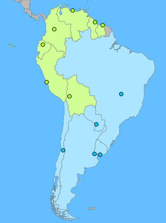
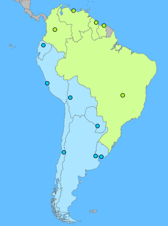
In my example, I am trying to form 2 groups (k = 2). Again I use the capitals to represent the location of each country, and I start by randomly setting the two centroids at Lat/Long {0, -70} (near the border between Colombia & Brazil) and {-20, -50} (southwest of Brasilia).
The next step is to check whether the capitals are closer to Point 1 or Point 2.
| Country | Capital | Distance (km) | Group | |
|---|---|---|---|---|
| Point 1 | Point 2 | |||
| Argentina | Buenos Aires | 4033 | 1822 | 2 |
| Bolivia | La Paz | 1846 | 1955 | 1 |
| Brazil | Brasília | 2991 | 518 | 2 |
| Chile | Santiago | 3721 | 2530 | 2 |
| Colombia | Bogotá | 684 | 3796 | 1 |
| Ecuador | Quito | 948 | 3804 | 1 |
| Guyana | Georgetown | 1516 | 3111 | 1 |
| Paraguay | Asunción | 3111 | 980 | 2 |
| Peru | Lima | 1548 | 3016 | 1 |
| Suriname | Paramaribo | 1771 | 2931 | 1 |
| Uruguay | Montevideo | 4131 | 1757 | 2 |
| Venezuela | Caracas | 1216 | 3861 | 1 |
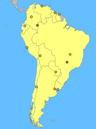
This gives us the preliminary grouping of the capitals/countries. The next step is to recalculate the two centroids based on the two groups.
- Point 1 (green): {-0.1435, -68.2838}
- Point 2 (blue): {-28.7952, -58.1563}
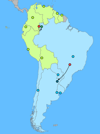
You can see how the centroids move and "improve". Now repeat the calculation of the distances between the capitals and the two new centroids:
| Country | Capital | Distance (km) | Group | |
|---|---|---|---|---|
| Point 1 | Point 2 | |||
| Argentina | Buenos Aires | 3967 | 646 | 2 |
| Bolivia | La Paz | 1819 | 1707 | 2 |
| Brazil | Brasília | 2831 | 1787 | 2 |
| Chile | Santiago | 3713 | 1296 | 2 |
| Colombia | Bogotá | 833 | 4086 | 1 |
| Ecuador | Quito | 1139 | 3844 | 1 |
| Guyana | Georgetown | 1364 | 3959 | 1 |
| Paraguay | Asunción | 3022 | 392 | 2 |
| Peru | Lima | 1638 | 2701 | 1 |
| Suriname | Paramaribo | 1602 | 3867 | 1 |
| Uruguay | Montevideo | 4058 | 697 | 2 |
| Venezuela | Caracas | 1192 | 4467 | 1 |
You can see that Bolivia is now switched to Group 2. Keep repeating the same until the centroids and the groupings do not change anymore, and now you have the two clusters.
Spectral Clustering
So far the two methods above are purely based on the distance between the country capitals. We have not considered the country border (edges) yet. The issue is that in the case of non-bordering countries that are near each other (e.g. Djibouti & Yemen), these will likely be put into the same cluster although they are 7 edges apart.
To properly consider the relationship between countries based on borders, we do need to look at the edges and turn the countries into a graph as I mentioned earlier. (Again for simplicity sake, I am ignoring France and Panama)
Spectral clustering requires some basic understanding of linear algebra which I will not go into the details of the maths behind it (I don't know that well myself either 😅). Rather I would show you how it is done. In this method, there are three steps involved:
- Construct a Laplacian matrix representation of the graph.
- Compute the eigenvalue and eigenvector of the matrix.
- Apply the eigenvector to the nodes to form the clusters.
Let's see how it is done. In simple term, the Laplacian matrix is a table of numbers that represents the above graph. You can read the Wikipedia page to learn more, but basically the formula is L = D - A, or put simply, a table where the diagonal is the number of edges (number of bordering countries), and the rest of the numbers are either 0 if they don't border each other, or -1 if they do. (Note that all rows and columns sum up to 0). So for South America, the Laplacian matrix looks like this:
| AR | BO | BR | CL | CO | EC | GY | PY | PE | SR | UY | VE | |
|---|---|---|---|---|---|---|---|---|---|---|---|---|
| Argentina | 5 | -1 | -1 | -1 | 0 | 0 | 0 | -1 | 0 | 0 | -1 | 0 |
| Bolivia | -1 | 5 | -1 | -1 | 0 | 0 | 0 | -1 | -1 | 0 | 0 | 0 |
| Brazil | -1 | -1 | 9 | 0 | -1 | 0 | -1 | -1 | -1 | -1 | -1 | -1 |
| Chile | -1 | -1 | 0 | 3 | 0 | 0 | 0 | 0 | -1 | 0 | 0 | 0 |
| Colombia | 0 | 0 | -1 | 0 | 4 | -1 | 0 | 0 | -1 | 0 | 0 | -1 |
| Ecuador | 0 | 0 | 0 | 0 | -1 | 2 | 0 | 0 | -1 | 0 | 0 | 0 |
| Guyana | 0 | 0 | -1 | 0 | 0 | 0 | 3 | 0 | 0 | -1 | 0 | -1 |
| Paraguay | -1 | -1 | -1 | 0 | 0 | 0 | 0 | 3 | 0 | 0 | 0 | 0 |
| Peru | 0 | -1 | -1 | -1 | -1 | -1 | 0 | 0 | 5 | 0 | 0 | 0 |
| Suriname | 0 | 0 | -1 | 0 | 0 | 0 | -1 | 0 | 0 | 2 | 0 | 0 |
| Uruguay | -1 | 0 | -1 | 0 | 0 | 0 | 0 | 0 | 0 | 0 | 2 | 0 |
| Venezuela | 0 | 0 | -1 | 0 | -1 | 0 | -1 | 0 | 0 | 0 | 0 | 3 |
The next step is to find the eigenvalue and eigenvector of the above matrix. In simple term, the eigenvector (v) is a special vector of a matrix (T) such that multiplying by it will scale the vector linearly by a constant eigenvalue (λ), i.e. Tv = λv. You can think of it as a way to enlarge a photo without distorting it.
There is no magic formula to calculate the eigenvalue and eigenvector of a matrix. The simplest way is to use the Excel Goal Seek tool under What-If Analysis to iterate until it finds the best possible answer. I will not go through the method here, but you can check out YouTube videos such as this and this on how this can be done. (Or if you are already using Matlab then you don't need me to teach you how).
With that, it calculates the second smallest eigenvalue of our Laplacian matrix to be 1.08958 (you don't want the eigenvalue of 0 which is useless to us), and the corresponding eigenvector is
| -0.83 |
| -0.82 |
| 0.22 |
| -1.21 |
| -0.02 |
| -0.75 |
| 1.96 |
| -0.75 |
| -0.66 |
| 2.39 |
| -0.67 |
| 1.13 |
Applying the eigenvector to our list of countries and sorting it, we have a group of countries with negative numbers and another group with positive numbers. i.e.
| Group 1 | Group 2 | ||
|---|---|---|---|
| Chile | -1.21 | Brazil | 0.22 |
| Argentina | -0.83 | Venezuela | 1.13 |
| Bolivia | -0.82 | Guyana | 1.96 |
| Paraguay | -0.75 | Suriname | 2.39 |
| Ecuador | -0.75 | ||
| Uruguay | -0.67 | ||
| Peru | -0.66 | ||
| Colombia | -0.02 |
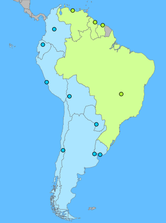
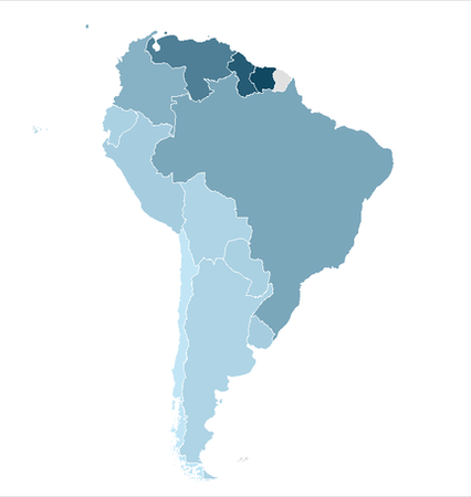
As you can see, since the South American countries are all well interconnected, it is difficult to form two distinct clusters. But when I apply the same calculation to both North and South America, the result is much more obvious.
| Group 1 | Group 2 | ||
|---|---|---|---|
| Uruguay | -0.504 | Costa Rica | 0.103 |
| Paraguay | -0.501 | Nicaragua | 0.359 |
| Argentina | -0.501 | Honduras | 0.599 |
| Suriname | -0.499 | El Salvador | 0.680 |
| Chile | -0.497 | Guatemala | 0.732 |
| Bolivia | -0.495 | Belize | 0.794 |
| Guyana | -0.492 | Mexico | 0.821 |
| Brazil | -0.485 | USA | 0.902 |
| Peru | -0.472 | Canada | 0.944 |
| Venezuela | -0.469 | ||
| Ecuador | -0.451 | ||
| Colombia | -0.410 | ||
| Panama | -0.157 |
Modularity Clustering
Modularity is a way to quantify how closely related the nodes are within a cluster. In this method, we try to maximise the combined modularity score of the clusters so that we are putting closely related nodes together rather than unrelated ones.
The formula for calculating modularity looks quite daunting but it is actually much simpler than what it seems. Let me explain:

where
Q = modularity score, what we are trying to calculate for our clusters
m = total number of edges in our graph, i.e. total number of country borders
Aij = adjacency score between node i and j, 1 if node i borders node j, or 0 if they don't
γ = resolution factor, equals to 1 by default unless you want to add weight to the expected probability of node i and j being connected
ki and kj = degrees of node i and j. In the standard case where we treat all borders equal, this is the number of borders (edges) that country i and j (node i and j) have.
δ(ci, cj) = Kronecker delta, just a fancy way to say that if i = j then it is 0 else 1, i.e. only add up when country i and j are different, e.g. count Argentina-Chile, not Argentina-Argentina.
So how does it work? Let's say we want to examine the modularity score of the two clusters formed by spectral clustering above. First there are in total 23 edges in the graph (23 borders, m=23). For Group 1, we need to sum up for all node pairs, e.g. for Chile - Argentina:
- Aij = 1 (they do border each other)
- ki = 3 (Chile borders 3 other countries)
- kj = 5 (Argentina borders 5)
Aij - (ki kj / 2m) = 1 - (3 x 5) / (2 x 23) = 0.674
And for say Colombia - Bolivia,
Aij - (ki kj / 2m) = 0 - (4 x 5) / (2 x 23) = -0.435
So on so forth. The calculation gives Q1 = 0.0681 and Q2 = 0.0647, and hence a total score of 0.133.
Let's say I want to even out the number of countries in each group so I move Colombia to Group 2. Redoing the same calculation gives a new total score of 0.148, so it is not a bad idea! And if I want to have exactly 6 countries in each group so I move Peru to Group 2 too, the calculation gives a new total score of 0.124. So I should probably think twice before doing that.
Considerations
There are many other methods of clustering, some are focusing on the finding the nodes that are closely connected to each other, others are trying to find nodes with similar topology, e.g. countries like Brazil, Germany, DR Congo are similar as they tie other countries together. Some methodology is limited to finding a small number of clusters (e.g. 2) and fails when trying to form larger number of clusters (e.g. 10 groups of COTW), or when there is no clear distinction among the nodes to form a cluster, or unable to ensure each cluster has the similar number of nodes.
Another consideration comes to how we define the edges, especially for island countries. There are only 4 bridges/tunnels in the world that connect non-neighbouring countries together, namely:
- United Kingdom - France: Channel Tunnel
- Denmark - Sweden: Øresund Bridge
- Bahrain - Saudi Arabia: King Fahd Causeway
- Singapore - Malaysia: Johor Causeway and others
For others, how should the edges be defined? For example, should Japan be connected to Russia, and Taiwan? and South Korea? Or should United States be connected to Russia? The Bahamas? Kiribati? How about the territories (e.g. Canada-Denmark)? And don't get me started on Cyprus (to Greece or not to Greece, that is the question 😄).
Besides, should all borders and edges be treated equal? They are in my calculation above, but not all borders are the same, e.g. there is no land crossing between Colombia and Panama. Some bordering countries are culturally and geopolitically very far apart, e.g. Russia-North Korea, China-Afghanistan.
Final Thoughts
After reading all these, you may ask the question why? Why do we spend so much effort into clustering? It is very obvious to anyone that North and South America form two different groups without all these calculation. But we cannot always do it manually and visually, especially when the number of nodes is huge and the edges are complex.
The application of clustering goes far beyond countries and maps. What if these countries are high-schoolers and the graph represents their social network on TikTok? Should I push ad selling American goods to the popular Brazilian influencer who has so many connections? Clustering can help identify how genes are grouped together, or help AI identify objects in photos, or identify fraudulent activities in your credit card transactions, or for Natural Language Processing (NLP) to understand words (or dog barks) with similar meanings. And the opportunities are endless.
As you can see, doing these calculation manually is almost impossible (it's tedious and error-prone). People would write Python scripts and let machine learning do the hard work. If you find this interesting, study Discrete Maths and Data Science in university and your future is bright!
Advertisement time: I do have few quizzes here with graphs, have fun with these!
I can’t help but think about how Topological Data Analysis tools must be very applicable here too. I imagine you could construct a Rips Complex based on various geopolitical similarities. I’m not well versed enough in TDA to know how to interpret the persistent homology, but I’m sure there’s an R package that could easily do all the heavy lifting for you!